The Jimp 2 version 0.083 User Guide
Jimp 2 Citation
All publications and/or presentations that result from the use of Jimp 2 should contain the following references: Hall, M. B.; Fenske, R. F. Inorg. Chem. 1972, 11, 768-779. Manson, J.; Webster, C. E.; Pérez, L. M.; Hall, M. B. http://www.chem.tamu.edu/jimp2/index.html
Installing Jimp 2
Installing on Windows
To install Jimp 2 on windows, run the installer, which will be named "jimp2_X.XXX_install.exe". Administrator privileges are required to install to the default location (C:\Program Files\Jimp2), but if you don't have those priveleges, it should still be possible to install Jimp 2 to your home directory. The only hiccup is that to run Jimp 2, you must be a power user (a user with somewhat expanded priveleges), otherwise it will crash while opening.
Installing on Linux
To install Jimp 2 on Linux, download the provide rpm and use your favorite rpm installer.For the POV-Ray Dialog to work, POV-Ray , the Persistence of Vision Raytracer, must also be installed.
Using Jimp 2
In Jimp 2 there are three distinct areas with which the user can interact. These are the Menu Bar, the Tree View, and the OpenGL View. As well, everything can be controlled through scripting.
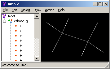
OpenGL View
Most of one's time will be spent staring at the OpenGL View, so we will cover it first.
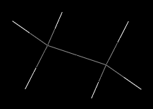
In the OpenGL View it is possible to perform various simple actions on the objects that one sees. One can drag a selection box to select a number of atoms and bonds at the same time, one can click to select single atoms or bonds, one can move atoms, and one can move the view.
Below is a full list of the commands that can be given to the OpenGL View. LMB, RMB, and MMB mean the left, right, and middle mouse buttons respectively.
| RMB+Drag | Rotate view. If initiated in corner, rotation is around view axis. |
| LMB | Select nearest atom or bond within 1 angstrom radius. |
| RMB | Popup menu. |
| LMB+Drag | Select atoms within drawn box. |
| LMB+Shift | Toggle selection of nearest atom or bond within 1 angstrom radius. |
| LMB+Drag+Shift | Toggle selection of atoms within drawn box. |
| MMB+Drag LMB+Drag+Shift+Alt |
Translate the view. |
| LMB+Ctrl | Zoom in or out -- move along up/down. |
| RMB+Drag+Ctrl | Rotate selected atoms. |
| MMB+Drag+Ctrl RMB+Drag+Ctrl+Shift |
Translate selected atoms. |
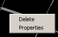
As well as having the above list of commands, a couple of other actions can be performed through the popup menu from right clicking. One can delete the selected objects, or one can bring up the properties dialog.
Measuring
There are three types of measurements that can be performed. Distances, angles, and dihedrals can be measured, and they all use the same interface.To begin measuring select the menu bar item "Draw -> Measure Begin/End" which has the shortcut key Ctrl-E. Once one has initiated the measuring mode, click on a sequence of atoms, then end the measurement in the same way that it was started. If two atoms were clicked on, a distance measurement is created; three atoms, an angle; and four atoms, a dihedral. Angle and dihedral measurements are reported in degrees; distances in Angstroms.
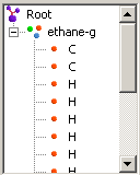
Tree View
The Tree View shows and allows the manipulation of the hierarchy of objects in one's Jimp 2 session. There are some objects that can not be selected through the OpenGL View and must be selected with the Tree View.
Ordering of the list
The list of children of a node can be sorted, or the node can be sorted recursively. When the list is sorted, objects are grouped together. All objects except for bonds are put higher in the list than atoms. Bonds are put at the very end. Atoms are ordered by atomic mass, with the heaviest atoms put at the top of the list. Bonds are also ordered by the mass of the connected atoms. All other objects are sorted alphabetically and numerically in a natural sort of way, such that "field 1", "field 2", and "field 10" will be in the expected order.When objects are added to a node, they are not automatically put into sorted order. Rather, atoms and bonds are put at the end of the list and everything else is put at the top.
The icons
Each type of object has its own icon so that one can easily tell them apart. The list of icons follows:-
 - The root node
-
 - An atom
-
 - A bond
-
 - A node
-
 - A measurement
-
 - A field
-
 - A surface
Moving objects
Objects can be moved by dragging them onto the object to which one wants them to become a part. Different objects will allow different sorts of objects to be attached to them. For example, a node can have anything under it, but a field can only have surfaces as its children and will not accept anything else being dragged onto it.
The popup menu

The popup menu comes up when one right clicks in the Tree View. The following sections will explain the options presented in the popup menu in detail.
The workarea
Any object can be set as the workarea, but it only makes sense to set a node as the workarea. Only objects within the workarea can be selected through the OpenGL View. As well, there are some actions that are performed on every atom in the workarea, or if no other objects are selected, the program assumes that they should be performed on the entire workarea. Center View (Ctrl-R) is an example of this behavior. Also, the background color of the 3D renderings is the same as the color of the object that is set as the workarea.
Visibility
Visibility has three basic states: Normal, Always Hidden, and Always Shown. The visibility of an object can be changed by right clicking on it and selecting the appropriate popup menu item. As well, the current workarea is always considered to be visible. The visibility of an object will affect that of its sub-objects as well as the object itself. This makes it easy to hide or show an entire molecule or parts of it by organizing the molecule into nodes. An object should not be set as both hidden and shown, because only one will be honored.
-
- A visible bond
-
 - A hidden bond
-
 - A bond that will always be shown
Creating nodes
A new node can be created either through the popup menu or by using the hotkey Ctrl-N. With the popup menu the node will be attached to what was clicked on. Ctrl-N will attach the node to the root and set it to be the current workarea.
Menu Bar
The Menu Bar will directly perform a few actions, but its two primary purposes are to intercept certain special keystrokes, such as Ctrl-S to save, and to provide access to various dialogs.

The special keystrokes
The list of hotkeys is as follows:| Ctrl-O | Open |
| Ctrl-S | Save |
| Ctrl-Shift-S | Save As |
| Ctrl-Z | Undo |
| Ctrl-Shift-Z | Redo |
| Ctrl-X | Cut |
| Ctrl-C | Copy |
| Ctrl-V | Paste |
| Ctrl-A | Select All |
| Ctrl-Shift-D | Deselect |
| Ctrl-I | Invert Selection |
| Ctrl-H | Hide (toggles) |
| Ctrl-Shift-H | Hide Hydrogens (toggles) |
| Ctrl-L | Script Dialog |
| Ctrl-Del | Delete |
| Ctrl-R | Center View |
| Ctrl-E | Begin/End Measurement |
| Ctrl-D | Begin/End Atom Drawing |
| F5 | Refresh All |
Cut, Copy, and Paste
Copying and pasting should work as expected, but the actual mechanism behind it is slightly different than most programs. When anything is cut or copied, a file named "copy_buffer.jm2" is written to the Jimp 2 directory. When pasting, this file is then read from disk and then the selected objects are added to one's session. This means that objects can be copied and pasted between concurrently running processes of Jimp 2, or even after rebooting.
Properties Dialog
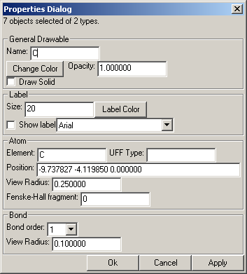
The properties dialog has several stackable components. Only the components relevant to the selected objects are shown. At the very top the dialog box says how many objects and of how many types are selected.
Whenever new objects are selected, the properties dialog is updated to reflect the current selection. It may be confusing how the items are assigned their default values when multiple items are selected. Not all of the different values of the objects can be easily shown, so only one of the objects is used. Never fear though; only the properties that one modifies will be applied to the different objects.
General Drawable
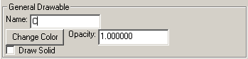
Name refers to the name of the object.
The color button will allows one to change the color.
Opacity will change the opacity of the object. In the OpenGL View this only affects text, but with POV-Ray anything can be transparent.
Atom
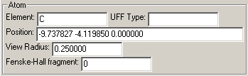
When changing the element, the color, label, and other properties intimately related to the element are also changed to the default values for that element.
The UFF type is used in the minimization of the structure of a molecule, and when no type is specified, a default type for that atom will be assigned.
The view radius is the radius that will be used for the sphere of the atom when drawn solid. If you would like to have a view of the molecule where the atoms do not show, such that there are only cylindrical bonds with rounded ends, set the view radius of all atoms to be the same as the bond view radius.
Fenske-Hall Fragment refers to which fragment the atom will be considered to be a part when doing fragment analysis with the Fenske-Hall Dialog. Numbers greater than one can be used to set a fragment. Zero indicates that the atom is not a part of any fragment (or is an independant fragment if one thinks of it that way).
Bond
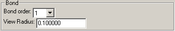
Set the bond order and radius of the bond when drawn solid.
Label
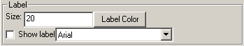
Label refers to what text will be shown for this object. Some objects, like measurements, can not have the label directly changed.
Size refers to the pointsize of the text drawn. This is for the native screen resolution and will be scaled when doing a screen grab to keep the same proportions.
Label color changes the color of the label.
Show label will toggle the showing of the label.
The combo box with different font names allows one to change the font used for the label.
Field
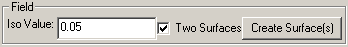
The iso-value is the field strength that the surface will occupy. If the two surfaces box is checked, then a surface will also be created for the opposite signed iso-value. Unlike most properties, the surface(s) will be created immediately when the "Create Surface(s)" button is pressed.
Measure
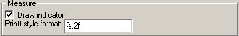
The indicator is the dotted line showing where the measure is. The "Draw indicator" check box determines if it is drawn.
The printf format allows changing how the label is made for a measure. For a full explaination of how formatting with printf works, see this reference . Obviously, the number passed in to printf is a float (real number), so do not use "%s" for the format. If one desires, one can add text here also, as in, "The distance is %.3f Angstroms".
Fenske-Hall Dialog
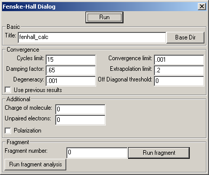
The big friendly "Run" button at the top will perform a basic SCF calculation with no fragments. The results from the calculation will be put into a directory (folder) with the same name as the title. This directory will be in the directory specified through the "Base Dir" button. If no base directory has yet been specified, then the current working directory will be used. What the working directory is depends on the operating system and how exactly Jimp 2 has been run, so unless one is familiar with this aspect of ones operating system, it is a good idea to explicitly set the base directory.
Under the "Additional" section it is possible to set the charge of a molecule and the number of unpaired electrons. Before a calculation is run, these values are checked to make sure that they agree, and if they do not, a message box will appear. It is assumed that the unpaired electrons are all in the highest occupied orbitals. If the polarization box is checked, then a basis set with polarization functions is used for main group atoms.
Interpreting the output files
Converging tricky calculations
Fragment analysis
First, each individual fragment must have an SCF run separately, then one can perform the fragment analysis on the whole molecule, which will give the contribution of the individual fragments to the orbitals of the entire molecule. If there are atoms that should be a fragment of their own, such as a metal, set those atoms to fragment zero. Zero is a special fragment that is no fragment at all.One thing to keep in mind when doing fragment calculations is that the charge and unpaired electrons must be correctly set for each fragment, and then for the entire molecule when doing the last step in fragment analysis. Fragments often have a charge other than zero, so this is of special concern.
A short tutorial on how to run and visualize fragment MO's was created by Edwin Webster: Download the 111-trifluoroethane.log and 111-trifluoroethane.msi files and follow the instructions in 111-trifluoroethane.log.
Moplot Dialog
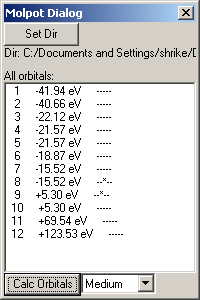
When a Fenske-Hall calculation is completed, the directory of the Moplot Dialog is automatically set to be the same thing. However, if one is returning to a calculation that has been completed previously, it is possible to manually point Moplot to the completed Fenske-Hall calculation through the "Set Dir" button.
An orbital can be made viewable either by double clicking on it or by selecting a number of orbitals and clicking the "Calc Orbitals" button.
Moplot creates a 3D grid where each point in the grid has a value representing the strength of the field at that point. Grids of higher resolution take more time and memory to compute and store, so Jimp 2 allows one to choose what field density should be calculated. Each density is twice as great as the previous in each dimension, meaning that it has eight times number of data points. The names for the densities are: Chunky, Coarse, Medium, Fine, and Ultra-Fine. The density at which the calculations will be performed and the results which will be displayed is selected by the combo box in the bottom right corner.
Each line in the list of orbitals has three parts. The first is the number of the orbital. The second is the energy of the orbital (the lower the value, the more likely it is to be occupied by electrons). The third is a series of dashes and stars indicating whether a field has been calculated for that orbital and at what densities. A dash (-) means that no field has yet been calculated and a asterisk (*) means that it has already been calculated. The represented densities increase from left to right; the leftmost is chunky and the rightmost is ultra-fine.
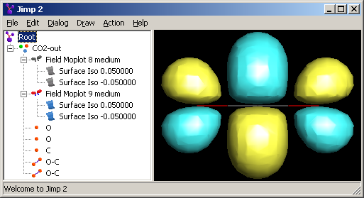
The Moplot Dialog provides a lot of functionality, but for finer grained control of how what is displayed, one has to turn to the Tree View. If one looks above, one will notice that the fields for two orbitals of CO2 and their coresponding surfaces have been calculated. The 8th and 9th orbitals (valence) have been calculated at medium resolution. Because 8 is grayed out, it means that the orbital shown is the 9th. Using the hide/show functions of the popup menu it is possible to show multiple fields, none, or to show only specific surfaces.
The surfaces, once they have been calculated, are independant of the field from which they were generated. This means that one can move them out of the field node or even delete the field from which they were created. For example, if one is making a presentation, one may want to delete the field, because it takes a lot of memory. The 10th orbital of C02 with the field took 393 KiB of space and without it took 281 KiB of space saved as a JM2 file. It is possible to select a surface and change its properties from the Properties Dialog, accessed through the popup menu, one can change its color and other attributes.
What exactly is needed to do a calculation
To generate a field with Moplot, only the vector file, named "vector.vec", from the Fenske-Hall calculation is needed. However, for the Moplot Dialog to work correctly, the file "oren.txt", which has the orbital energies, is also required. If one has only the vector file, it is still possible to generate a field using the script function directly.
Script Dialog
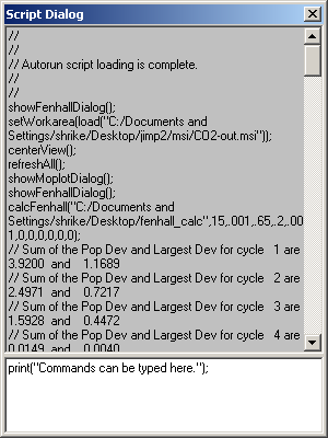
The Script Dialog is a view into what is going on inside of Jimp 2. Every action that can be done through dialogs and such can be done through the scripting language. In fact, every action is done through the scripting language; and when it is done, the command is logged both to a file and to the script window. It is also possible to execute ones own script commands through the bottom pane of the Script Dialog. Pressing Enter will run the command, and if multiple lines are needed, one can press Ctrl-Enter to insert a line break. As well, one can paste up to 32 KiB of text. If one has a script that is larger than that, use the script function exec("scriptfile.ts") to run a specific script saved in a file.
The specifics of scripting are discussed later in the guide.
Grab Screen Dialog
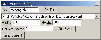
The Grab Screen Dialog allows one to save an image to a file of exactly what is shown in the OpenGL View. One may also specify arbitrary resolutions at which the image will be produced. This can be very useful for making presentation or print quality pictures, because very high resolutions are allowed. Think of printing a 8.5"x11" graphic at 1200 dpi, which requires a 10200x13200 pixel image. No problem; well, except that the uncompressed image will take about 385 MiB of memory while it is being composited, so one's computer may chug for a while.
The "Set Dir" button sets to where the image file will be written, and the title is the name of the file, minus the extension which is automatically added. One may either directly specify the width and height of the image, or, by pressing "Get Size", one can have the dialog set the width and height. The size will be based off of the current size of the OpenGL View area and is multiplied by the size factor, which can be a fractional number such as 1.5, if desired.
The only difference in this dialog from the Povray Dialog is that one can specify the format of the output image. Each option has a brief description next to it, and it is recommended to use the PNG format (which also is the default). Many people are inclined to use JPEG, because they are more familiar with it, but the compression method used in the JPEG is only really suitable for photographs that are not expanded much.
Povray Dialog
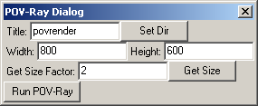
The Povray Dialog is nearly identical to the Grab Screen Dialog. The only difference is that one does not get an option of what format to save the image. The saved image is always a PNG.
In order to render an image with POV-Ray one must first make sure that POV-Ray is installed. The installation of POV-Ray is also covered in the installation section of this guide.
Calculate Bonding Dialog
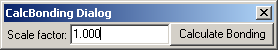
Bonds will be created between the selected atoms or all atoms if none are selected. Whether the bond exists and if it does what the order of the bond should be is determined from the van der Waals radius of the atoms. The scale factor can be modified to make bonds more or less likely to form than the default of 1. A fair bit of time was spent getting this feature to operate quickly; and it really does not take much time, even on all the atoms in a large protein.
Scripting
Scripting can be a very useful tool, and if one finds oneself using Jimp 2 a lot, it may be a good idea to play with the scripting language. One reason is that scripting allows for the automation of common tasks. Another is that there are a few hidden features that are only accessible through the scripting language. This may be because there is no easy way to make the function available through the GUI or that it just has not yet been implemented! In general the script function is written to do things before the GUI, because eventually the GUI will have to call the script (and because GUI programming is not fun).
The history of Terra Script
The language used for scripting in Jimp 2 is called Terra Script, which was written by Josiah Manson. The language was originally written for a game that the author eventually lost interest in making, called Terra Vive. Terra Script was then incorporated as a server side scripting language for a toy web server, again coded by Josiah Manson. Then, when Josiah started working on Jimp 2 it was decided that a scripting language would be really useful (Lisa Perez was especially clamoring for scripting). Josiah looked at various options and was not happy with the difficulty of embedding that many languages have. He was already familiar with Terra Script, so he decided to use it in Jimp 2.
The language
We will not be discussing the language too much, because it is fairly standard. Terra Script is based off of C, but has some differences. One difference is that like most scripting languages, variables don't have to be declared and have changeable type. While C uses semi-colons to separate parts of a 'for loop', e.g.,for (int i = 0; i < 10; i++){}
, the equivalent in Terra Script is,
for (i = 0, i < 10, i++){}
Also, all code blocks must be contained in curly braces. Accessing arrays looks
somewhat different as well. In C, the ith element in the array a is
a[i]and in Terra Script it is
a@i
The language is limited in plenty of other ways as well, but it gets the job done. There should be some scripts included with the program to give a better feel for the language.
Autorun
In the directory to which Jimp 2 is installed, if there is a file named "autorun.ts", it is executed every time that Jimp 2 is run. In this file it is possible to set defaults and to do basically anything that can be done in the program normally.
The log
Whenever anything happens in Jimp 2 it was motivated by a script command. All of these commands are written to a log file named "log.ts" in the Jimp 2 program directory. This log can then be replayed in a new session.